Tutorial: train a model
In this tutorial we will show you step-by-step how to train a binary classification model with the help of MyAutoML.
If you already have a local copy of MyAutoML including a working environment you may head over directly to Configuration. Otherwise, start with correctly installing MyAutoML.
Installation
Before we start you might wonder: what is Cookiecutter? Cookiecutter is a CLI tool that allows you to easily create a project structure including folders, scripts and documents. It is a way to save time if you find yourself creating and copy-pasting the same folders and scripts over time. A brief introduction can be found on medium. You can install Cookiecutter with pip.
pip install cookiecutter
If you already have Cookiecutter installed make sure it is up to date since we will use the –directory option. Note that we intend to move the cookiecutter to a separate repository, but for now it’s still in a directory within this repository. More information on the installation of Cookiecutter can be found here. Once installed, move to the folder where you want to store MyAutoML and execute the following command.
cookiecutter https://github.com/myautoml/myautoml.git --directory="cookiecutter/binary_classifier"
You will be prompted with a few questions regarding the project, this is a convenient feature of Cookiecutter to customize the new project to your wishes. When finished you are ready to create a new virtual environment.
A virtual environment allows you to install and use specific versions of Python and packages specifically for one project. This prevents cumbersome version conflicts when you run multiple projects from the same environment over time. More information on virtual environments can be found on real python.
Move to the /scripts folder and execute the following commands from your terminal.
conda env create -f environment.yml
conda activate <name_of_your_environment>
Configuration
MyAutoML comes with templated Python scripts and a config file, all meant to write as little custom code as possible, and to keep focused on what makes your project stand out: the data.
data
For this tutorial we are going to use the Bank Marketing Data Set from the UCI Machine learning repository. The official reference is:
[Moro et al., 2014] S. Moro, P. Cortez and P. Rita. A Data-Driven Approach to Predict the Success of Bank Telemarketing. Decision Support Systems, Elsevier, 62:22-31, June 2014
This dataset holds a typical marketing classification task, where we are interested in predicting whether a customer will respond to a marketing campaign yes or no. The independent variables are a mix of demographics (age), customer specific data (balance), and behavioural data (response to previous campaigns). For demonstration purposes we will only use 6 independent variables plus the dependent variable of the original dataset.
y |
age |
default |
balance |
housing |
loan |
poutcome |
|---|---|---|---|---|---|---|
False |
58 |
no |
2143 |
yes |
no |
success |
False |
44 |
no |
29 |
yes |
no |
unknown |
False |
33 |
no |
2 |
yes |
yes |
failure |
To transform this dataset to actual training data we need to modify scripts/data.py, specifically the
load_training_data function. Make sure to refer to the correct path of the dataset.
import pandas as pd
from pathlib import Path
from sklearn.model_selection import train_test_split


def load_training_data():
    df_path = Path('..') / 'data' / 'bank' / 'bank-full.csv'
    df = pd.read_csv(df_path, sep=';', usecols=['age', 'default', 'balance', 'housing',
                                                'loan', 'poutcome', 'y'])
    x = df.drop(labels='y', axis=1)
    y = df['y'].astype('category').cat.codes.astype('bool')

    x_train, x_test, y_train, y_test = train_test_split(x, y,
                                                        stratify=y,
                                                        test_size=0.2,
                                                        random_state=123)

    return x_train, y_train
Now that we have the training data, we need to shape it so it can be used for modeling.
pre-processing
There are 3 pre-processing steps we need to take:
Scale the numerical variables
Create numeric dummy variables for the categorical variables
Select the correct columns for each pre-processing step
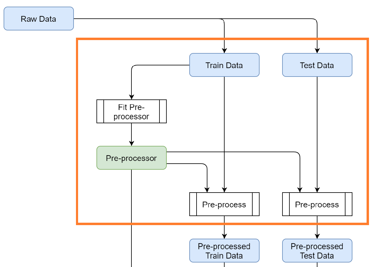
It is possible to perform these pre-processing steps with custom Python functions, but we opt to choose for a scikit-learn
pipeline. There are a number of advantages of using a pipeline, such as being able to fit the transformations on
the training data, and to apply these on the test data. This is an important step in building models but easily missed.
The official documentation of MyAutoML illustrates this nicely.
The pre-processor can be set in scripts/model.py, where an example pipeline is already shown in the get_preprocessor
function. We will overwrite the example with the following code.
def get_preprocessor():
    numeric_transformer = Pipeline(steps=[
        ('scaler', StandardScaler())])

    categorical_transformer = Pipeline(steps=[
        ('onehot', OneHotEncoder(handle_unknown='ignore'))])

    preprocessor = ColumnTransformer(transformers=[
        ('num', numeric_transformer, selector(pattern="age|balance")),
        ('cat', categorical_transformer, selector(pattern="default|housing|loan|poutcome"))]
    )

    return preprocessor
If any of this code is unfamiliar to you we can highly recommend watching these short videos on calmcode or read the official pipeline documentation.
estimator & hyperparameters
To be able to build a full model pipeline, MyAutoML also uses scikit-learn for its estimators. For this tutorial we will use logistic regression, but you can use any estimator from scikit-learn that is suited for binary classification.
To setup the estimator in scripts/model.py we need to retrieve a few things, which are all available in the
official LogisticRegression documentation.
module name: sklearn.linear_model
class name: LogisticRegression
hyperparameters: C, class_weight
This information is used in the get_estimator and get_params functions.
from sklearn.linear_model import LogisticRegression


def get_estimator(**params):
    estimator = LogisticRegression(**params)
    estimator_tags = {'module': 'sklearn.linear_model',
                      'class': 'LogisticRegression'}

    return estimator, estimator_tags


def get_params():
    estimator_params = {}
    search_space = {
        'C': hp.quniform('C', 0, 1, 0.0001),
        'class_weight': hp.choice('class_weight', [None, 'balanced'])
    }

    return estimator_params, search_space
Make sure that the keys from the search_space dictionary exactly match the names of the hyperparameters. The hp.
methods help to create a hyperparameter space which can be efficiently searched with hyperopt when training the model.
config.yml
The last part of the configuration is to setup the config.yml file. For now we increase the max_evals to 10 and set the shap_analysis to False. The rest of the settings will be discussed shortly, as they make more sense once we see the first results.
experiment:
  name: tutorial

model:
  name: tutorial

training:
  max_evals: 10

evaluation:
  primary_metric: roc_auc_cv
  metrics:
    - roc_auc
    - accuracy
  shap_analysis: False

prediction:
  stage: Production
Run & evaluate
You are now almost ready to run the train script. Make sure to make a copy of .env.general.template with the name .env.general.
The template shows the settings that are (may be) expected by the program, without containing any secrets such as passwords, so that it
can be committed to a git repository. You can update your personal and private settings in the .env.general file. Never commit your
.env.general (with passwords, etc.) to a git repository!
Change directory to the /scripts folder with
the MyAutoML environment activated and enter the following code to start the train script:
python train.py
If everything is setup correctly the script will start and you will see lots of logging statements in the terminal. Once
the training is finished we are ready to evaluate, and this is the part where MyAutoML really shines. Besides training the
model in an efficient manner with hyperopt, a lot of other things were taken care of by the train script:
Logging of the metadata of the estimator
Logging of the metrics
Creation of 5 typical binary classifier evaluation graphics
Creation of the model as .pkl file, including a config file to easily distribute the model
All these things are integrated in MLflow, so you can use easily use them via the UI. If you are not familiar with MLflow, it is an open source platform for managing the end-to-end machine learning lifecycle. Amongst other things, it keeps track of experiments to track and compare results. More information can be found on their website.
To open the UI you first need to start it via a new terminal. Please move to the scripts folder, activate the MyAutoML
environment, and execute the following command.
mlflow ui
Once you see the response in the terminal, head over to http://localhost:5000 and have a look. Note that we assume you are running this tutorial locally.
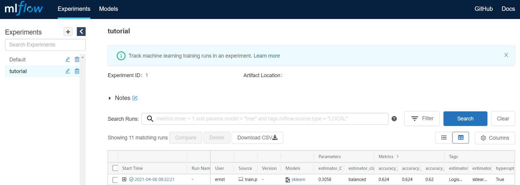
By pressing the + button you gain access to every training evaluation (config.yml -> max_evals), which contains
valuable information:
hyperparameter settings (complexity, balanced y/n)
evaluation metrics (accuracy in this case, specified for cv, train, and test)
tags (estimator class & model)
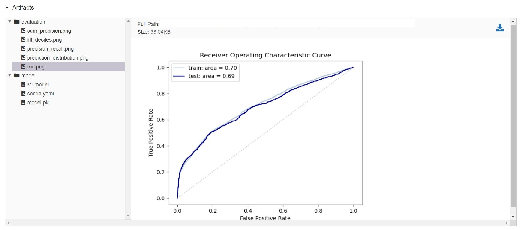
Although informative, it gets even better when you click on one of the runs. Besides ~20 evaluation metrics there is a special section at the bottom which is called Artifacts. This section contains the graphical outputs of the specific run, as well as the actual trained model.
There is more information available than we can describe here, so we highly recommend to take your time exploring the
experiment runs. Once finished, try to a different estimator and hyperparameter settings by adjusting the get_estimator
and get_params functions. When you run the train script again the results of these new evaluations will also become
visible in the UI, so you can easily compare which estimator and hyperparameter settings work best.
Wrapping up
Hopefully by now you have a better idea how MyAutoML works, and how it can help you to easily and efficiently train and compare binary classification models. In the following tutorial we will explain the next step in the modelling phase: prediction.